by Sukalp Muzumdar
(Disclaimer — The views and opinions expressed in this article are solely those of the authors and do not necessarily reflect the position of the authors’ employers.)
Given appropriate imaging, genotyping, and clinical data for a patient, can we accurately predict if they suffer from a specific type of cancer? Or determine if they will respond to targeted therapy? Can we accurately assess their risk of postoperative complications? These are some of the questions machine learning (ML) models are now helping answer in clinical data science. One of the key metrics used to evaluate the performance of these and indeed most ML models is the AUROC—Area Under the Receiver Operating Characteristic Curve. This article will explore AUROC’s historical context, clinical relevance, and its connections to other statistical metrics.
Background and History of the AUROC Metric
The AUROC metric has its origins in World War II, long before the rise of machine learning. Radar specialists developed the concept of Receiver Operating Characteristic (ROC) curves as a tool to assess radar systems’ effectiveness in distinguishing enemy aircraft from background noise (such as birds or weather anomalies). These specialists faced the challenge of balancing sensitivity (detecting enemy planes) with specificity (avoiding false alarms). The ROC curve became a useful tool to visualize this trade-off between true positives (correct detections) and false positives (false alarms).
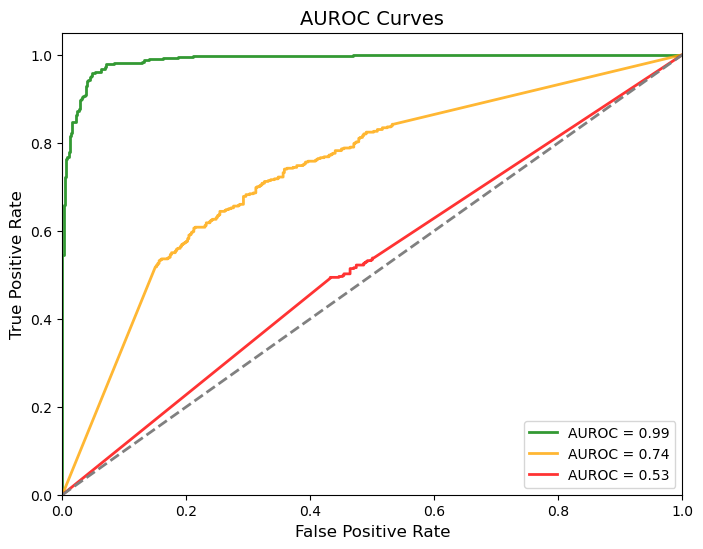
For instance, consider a radar system that detects 90% of enemy aircraft. However, it also falsely classifies 30% of migrating flocks of birds as planes. This system’s sensitivity (True Positive Rate, TPR) is high, but the false alarms increase the False Positive Rate (FPR). Plotting TPR against FPR across various classification thresholds creates the ROC curve.
AUROC as a statistical measure of separability
In today’s machine learning landscape, ROC curves have evolved into a powerful method for evaluating binary classifiers across various applications, from healthcare to finance. The Area Under the ROC Curve (AUROC) has become one of the most widely used performance metrics for its ability to summarize a model’s ability to distinguish between classes. But what does this metric fundamentally convey? Beyond simply being a number, the AUROC can be understood as a measure of separability—a gauge of how well a model can distinguish between positive and negative classes. Indeed, a more intuitive definition of the AUROC is the probability that a randomly chosen positive instance will be ranked above a randomly chosen negative instance. That is, if X represents a positive instance and Y represents a negative instance then we have –

This results from the AUROC being built up from individual classification thresholds for positive/negative instances, where the total area is effectively counting the fraction of positive-negative pairs where the positive score is higher. This makes the AUROC in essence, a rank-based separability statistic.
The Mann-Whitney statistic and AUROC
A commonly used rank-based statistical separability statistic is the U-statistic from the well-known Mann-Whitney U-test. The U-statistic can be expressed using the following formula, where Rx denotes the sum of the ranks of the positive class and nx denotes the number of positive instances –

From this formula, we see that we are adding up the ranks of the positive instances, and then subtracting the “intrinsic” ranking of these numbers by subtracting out the sum of the first nx natural numbers, which acts as a correction factor enabling us to only account for differences across groups. In essence then we are capturing the number of favorable pairwise comparisons across the two groups.
Now, to link this back to a probabilistic measure such as the AUROC, we need to divide it by a normalization factor, which in this case would be the total number of comparisons – if the number of positive and negative instances are nx and ny, this is the product nx*ny, representing all pairwise comparisons. Finally then, we arrive at –

which reveals an important relationship between these two metrics of separability, and establishes the AUROC as merely a normalized version of the Mann-Whitney U-statistic.
Cohen’s d and AUROC
Finally, coming to clinical trials, there is (justifiably so) great importance placed on not just statistically significant differences between arms, however also on the effect size, or the numerical value of the difference itself. A common metric which quantifies effect size is Cohen’s d, which is the standardized mean difference between two distributions. Simply, to calculate the Cohen’s d, the difference between the means of the conditions (μ1 – μ2) being compared is divided by their pooled standard deviations (σp), given by the following formula –

While Cohen’s d is often referred to as a measure of effect size, in essence it is quantifying the distance between the two distributions in units of pooled standard deviation (σp), which could be considered another statistical measure of separability.
Can we derive a relationship between the widely-used Cohen’s d and AUROC? In order to do so we have to make some assumptions about the distributions of the positive (X) and negative (Y) class scores – specifically that they are normally distributed, and have the same variance.
Given these assumptions are satisfied, then we have –

since X and Y are normally distributed, their difference is also normally distributed, with the mean being the difference between their means (μ1 – μ2) and the variance being the sum of the input variables’ variances (2σ2).
We can then also re-arrange the terms of the AUROC equation above as follows –

This new normally-distributed variable (X-Y) can be standardized/scaled by converting to a Z-score by subtracting the mean and dividing by the standard deviation, giving –

now we can put this Z value back into the to AUROC definition above,

removing out the zero from the RHS,

and since the normal distribution is symmetrically distributed, we can invert the sign and the inequality.

This probability can be expressed by the cumulative distribution function of the normal distribution Φ, and we can substitute back the difference of the means divided by the standard deviation as Cohen’s d, leading us to the final equation –

This derivation leads to a direct link between the AUROC and the Cohen’s d metric, given that the positive and negative score distributions are normally distributed and are homoscedastic (have equal variances). To demonstrate this relationship, I created a CodePen (link) where by playing around with the Cohen’s d between two distributions the effect it has on the AUROC (both theoretical based on the formula above, but also empirical by sampling from the two distributions) can be evaluated.
Wrapping up, we can see that the AUROC is a very versatile metric which encapsulates key separability information into one number and can be readily linked to other commonly-used statistical metrics of effect size and separability, demonstrating its utility beyond just evaluating the performance of a binary classifier. It is of course important to also recognize some of the limitations of relying solely on the AUROC. One major drawback is that AUROC does not reflect performance differences within specific ranges of the data, such as low or high threshold regions, which can be critical in clinical applications where false positives or false negatives are typically associated with uneven risks and costs. Additionally, AUROC can sometimes provide overly optimistic evaluations for imbalanced datasets where the minority class is the class of interest, as it does not take class distribution into account.

Leave a comment